Medium Features

Adaptive Sampling

Relevant code:

• src/core/Renderer.hpp :: SampleRecord
• src/core/Renderer.hpp :: generateWork
• src/core/Renderer.hpp :: dilateAdaptiveWeights

One of the noise reduction strategies I implemented is adaptive sampling. Adaptive sampling is a technique to distribute a sample budget to pixels based on an error metric that spends more samples where the perceptual error is larger. It attempts to make the error in the image uniform by moving samples from where they are wasted to where they are needed.
When implemented correctly, adaptive sampling can be very effective at making images converge quicker. It also enables a range of other noise optimizations - when adaptive sampling is enabled, any noise improvement that only helps a part of the image improves the image as a whole, since samples are automatically shifted around when part of the image becomes less noisy. This is not the case if no adaptive sampling is used.

My implementation is based on the paper "Robust Adaptive Sampling For Monte-Carlo-Based Rendering" by Pajot et al, which proposes an error metric that remains robust for incremental rendering and in the presence of outliers. In summary, they compute error weights based on the variance and median of the past N samples, reject the top 5% of errors and distribute samples according to the pixel error. They also interleave uniform sampling and adaptive sampling steps to remain robust if adaptive sampling fails.

I deviated from the paper in multiple places where their method did not work out. In particular, the median-error heuristic did not work robustly and tended to underestimate errors overall. I replaced it by a regular running mean/variance heuristic and was able to achieve good results.

One of the problem with adaptive sampling is that the error estimate itself is noisy due to the nature of the running variance. When a noisy heuristic is used to steer a noisy integrator, it is possible that errors amplifiy - undersampled areas such as caustics may be sampled less with naive adaptive sampling, since a pixel could have simply not received a high-intensity sample so far and would subsequently be classified as not noisy. In the initial phases of my implementation this was a big problem, and the "worst case" noise became even worse with adaptive sampling.

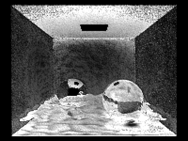
The "worst case" test scene I picked was the Cornell Box filled with water. This scene is challenging to render with forward path tracing due to the prominent caustics. The scene is shown below, without any adaptive sampling, rendered at 256spp:

Caustic scene without adaptive sampling

A renderer using the naive implementation of adaptive sampling with the above error heuristic for each pixel yields a result like this:

Caustic scene using bad adaptive sampling

Yikes! Clearly, this is not what we want. A first issue is that the error estimate for each pixel is very noisy in this scene, making the adaptive sampling very unreliable - some caustic pixels receive lots of samples, whereas the adjacent caustic pixel don't. To remedy this, I am grouping pixels into blocks of 4x4 pixels, each of which computes a single error estimate over the 4x4 pixel subregion. Since a lot more samples are used for each error estimate, this helps a lot with getting a more reliable estimate. When using this technique, we get a picture like this:

Caustic scene using block-based adaptive sampling

While this is a lot better, there are still apparent issues. If we are unlucky, an entire 4x4 block of pixels might compute a noisy error estimate that greatly underestimates the actual error. In that case we get an entire 4x4 block that is undersampled by the renderer, which causes noticable structured artifacts. Increasing the block size can make this situation less likely, although it also comes at great computational expense and decreases the adaptivity of the algorithm. Instead, I opted for a different solution: After computing the error weights, the error estimate is dilated by one block. That is, each block receives the maximum of its own error estimate and that of its neighbours. This is a completely empirical heuristic, but the intuition is as follows: Noisy light transport tends to be spatially coherent. If a pixel block is noisy, it is likely that the adjacent pixel blocks will also be noisy - this is true for caustics, specular higlights in DoF, glossy highlights and many more. In a way, the renderer automatically explores the blocks around a noisy block, and usually it will encounter noisy samples in the adjacent blocks too.
Applying this technique to the water cornell box gives this result:

Caustic scene using block-based dilated adaptive sampling

This is completely removes the structured artifacts and is also better than unadaptive sampling - despite the fact that the entire input scene is very noisy to begin with! In many scenes, not all parts of the image will have the same amount of noise, in which case adaptive sampling will be even more effective.

As a small bonus, here's an image showing the error estimate used to steer samples for this scene:

Error estimate

Microfacet reflection/refraction

Relevant code:

• src/core/bsdfs/Microfacet.hpp
• src/core/bsdfs/ComplexIor.hpp
• src/core/bsdfs/Fresnel.hpp
• src/core/bsdfs/RoughConductorBsdf.hpp
• src/core/bsdfs/RoughConductorBsdf.cpp
• src/core/bsdfs/RoughDielectricBsdf.hpp
• src/core/bsdfs/RoughDielectricBsdf.cpp
• src/core/bsdfs/OrenNayarBsdf.hpp
• src/core/bsdfs/OrenNayarBsdf.cpp

For this feature of the renderer, I implemented several microfacet models from literature.

The first two models come from the paper "Microfacet Models for Refraction through Rough Surfaces" by Walter et al. It gives a thorough background on microfacet theory for mirror microfacets and presents a new model for rough refraction.

I implemented both rough conductors and dielectrics including importance sampling following the paper. The phong, beckmann and ggx microfacet distributions are supported. I am also using the exact conductor Fresnel equations rather than an approximation. The user can either provide the complex, spectral refraction coefficients manually or select one of many built-in values from measured materials.

The images below show a conductor and a dielectric with a rough ggx distribution:

Rough conductor with ggx

Tungsten render without tonemapping

Mitsuba render

Rough dielectric with ggx

Tungsten render without tonemapping

Mitsuba render

The roughness value can also be modulated by a texture:

Rough conductor with textured roughness

Rough dielectric with textured roughness

For rough diffuse surfaces, I also implemented the Oren-Nayar model from the paper "Generalization of Lambert's Reflectance Model" by Oren and Nayar. I implemented their more accurate fit rather than the approximate qualitative fit.

The image below shows a rough diffuse material with high roughness:

Oren-Nayar BRDF

Tungsten render without tonemapping

Mitsuba render

Layered BRDF

Relevant code:

• src/core/bsdfs/MixedBsdf.hpp
• src/core/bsdfs/MixedBsdf.cpp
• src/core/bsdfs/SmoothCoatBsdf.hpp
• src/core/bsdfs/SmoothCoatBsdf.cpp
• src/core/bsdfs/PlasticBsdf.hpp
• src/core/bsdfs/RoughCoatBsdf.hpp
• src/core/bsdfs/RoughCoatBsdf.cpp
• src/core/bsdfs/RoughPlasticBsdf.hpp

For this medium feature, I implemented three BRDF models, two of which come in both smooth and rough variants, resulting in 5 new BRDFs.

The first model is based on the paper "Arbitrarily Layered Micro-Facet Surfaces" by Weidlich and Wilkie. It describes how to evaluate and sample materials consisting of multiple layers of rough dielectrics on top of a microfacet substrate. Their model ignores effects due to internal reflection, causing darkening for very rough subtrates.

Below is an image of a colored, rough conductor coated in a clear gloss dielectric:

Smooth dielectric coating on a colored rough conductor

Tungsten render without tonemapping

Mitsuba render

The dielectric layer optionally supports an extinction coefficient and a thickness parameter. These model the wavelength and angular dependence of light extinction as it moves through the dielectric layer. If we add extinction to the material shown above, we get a nice BRDF that looks similar to car paint:

Smooth, absorbing dielectric coating on a rough conductor

Tungsten render without tonemapping

Mitsuba render

One problem of the Wilkie model is that the effect of internal reflection is ignored. For very rough substrates such as a lambertian BRDF this can cause significant energy loss and darkening. For this reason, I also implemented a "plastic" BRDF, which is a specialization of the layered BRDF for a lambertian subsrate. Since the lambert model does only depend on the outgoing direction, we can analytically compute the effect of multiple scattering inside the dielectric layer through a geometric series. This considers all scattering events inside the material and gets rid of the darkening of the layered BRDF.

Below is an image of a plastic BRDF with a colored substrate:

Smooth plastic with colored substrate

Tungsten render without tonemapping

Mitsuba render

The plastic BRDF also supports specifying an absorption coefficient for the substrate:

Smooth plastic with a white substrate and an absorbing coat

For both the layered and the plastic BRDF, I also implemented a roughened version. Note that only rough reflection on the outer dielectric is considered. Refraction and internal reflection are still considered to be perfectly specular. Images of the rough versions of both BRDFs are shown below:

Rough, absorbing dielectric coating on a rough conductor

Rough plastic with white substrate and absorbing coat

Of course, we can also modulate the roughness by a texture. For the layered BRDF with a rough substrate, we also get the choice of roughening the substrate or the coat (or even both). The images below show this feature:

Rough, absorbing dielectric coating on a textured rough conductor

Textured rough, absorbing dielectric coating on a rough conductor

Textured rough plastic with colored substrate

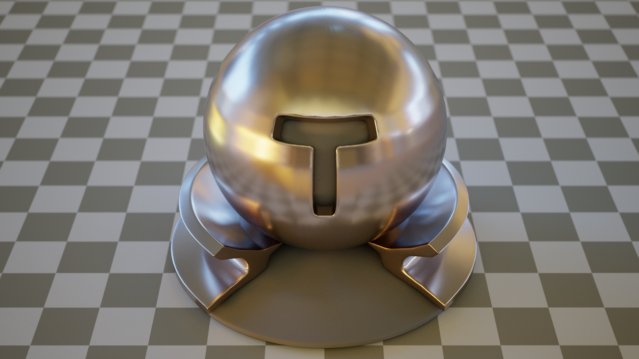
The final layered BSDF I implemented is the mixed BSDF. It blends between two arbitrary BSDFs based on a texturable mixture parameter. When sampling, it also performs multiple importance sampling between the two BSDFs.

Below is an image of a mixture BRDF of plastic and a rough conductor. It mimics the look of a gold coated ceramic:

Mixture of a gold and ceramic BSDF