Volumetric Path Tracing
Relevant code:
src/core/integrators/Medium.hppsrc/core/integrators/PhaseFunction.hppsrc/core/integrators/HomogeneousMedium.hppsrc/core/integrators/AtmosphericMedium.hppsrc/core/integrators/PathTraceIntegrator.hpp :: handleVolumesrc/core/integrators/PathTraceIntegrator.hpp :: volumeLightSamplesrc/core/integrators/PathTraceIntegrator.hpp :: volumePhaseSamplesrc/core/integrators/PathTraceIntegrator.hpp :: generalizedShadowRaysrc/core/integrators/PathTraceIntegrator.hpp :: attenuatedEmissionsrc/core/bsdfs/ThinSheetBsdf.hpp
For my advanced feature, I implemented Volumetric Path Tracing (VPT) in my renderer. It features homogeneous and atmospheric volumes, various phase functions, light sampling and phase function sampling with MIS as well as generalized shadow rays to battle noise.
Media in the renderer are always bounded by a primitive. The way this is implemented is that a BSDF can specify the media on the inside and the outside of the surface; whenever a ray transmits through the surface of a primitive, it will change media according to the BSDF. For convenience, if the BSDF does not specify any media, the medium of the ray is left unchanged.
Media can also be attached to the camera. For example, to render a foggy landscape, you would only have to attach a homogeneous medium to the camera. By default, the camera rests in a vacuum.
Media types
Currently, there are two different types of media implemented: The homogeneous medium, which has spatially constant extinction- and scattering coefficients, and the atmospheric medium, which is a specialized heterogeneous medium that can simulate planetary atmospheres. Most of this section will be about the homogeneous medium, since it is more general.
A medium implementation has to provide three operations: Sampling the distance to the next scattering location, sampling a direction at a scattering location, and computing the transmittance along a given ray. For the homogeneous medium, these operations can be implemented efficiently and analytically; for the atmospheric medium, more sophisticated handling is needed. See the sections below for details.
Homogeneous medium
Sampling a scattered direction and evaluating the transmittance is very simple in a homogeneous medium. Sampling a distance according to the extinction term is also not difficult for monochromatic media. However, for media with spectrally varying exinction coefficient, distance sampling can become difficult, since sampling according to just one of the color channels or the average extinction can introduce significant amounts of noise.
Luckily, there is a better solution, which I implemented in the renderer. Distance sampling according to a single color channel of the extinction coefficient can be seen as just one sampling strategy of the integrand. There are several sampling strategies available, however - one for each color channel. This means that we can randomly pick one of the color channels to sample a distance from, and then weight the result with multiple importance sampling using the pdfs of all the other color channels. The results achieved using this method are magnitudes better in noise for strongly spectrally varying media than just sampling with one strategy.
The homogeneous medium contains an optimization for the case when the scattering coefficient is zero (purely absorbing medium). It will never sample a distance inside the medium in that case.
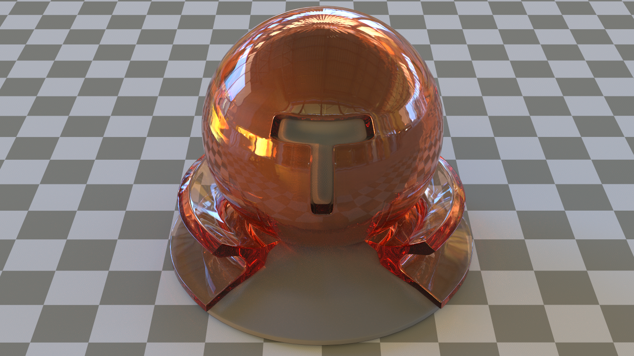
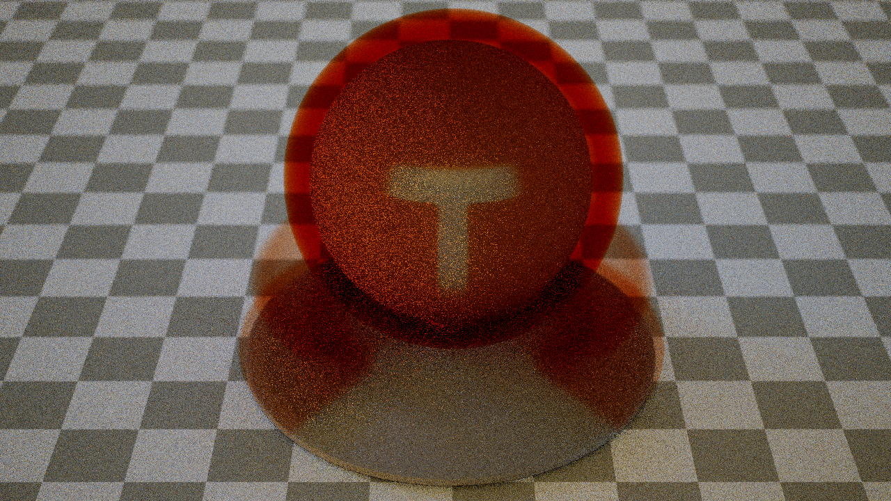
Below are two images of a purely absorbing, red homogeneous medium and a white scattering medium. The absorbing medium is encased in a dielectric boundary:

Red absorbing medium in a dielectric

Tungsten render without tonemapping
Mitsuba render
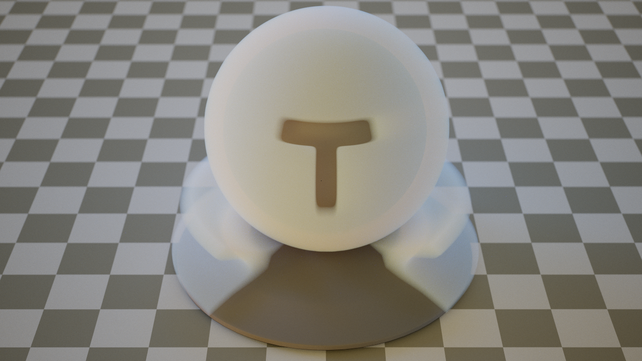
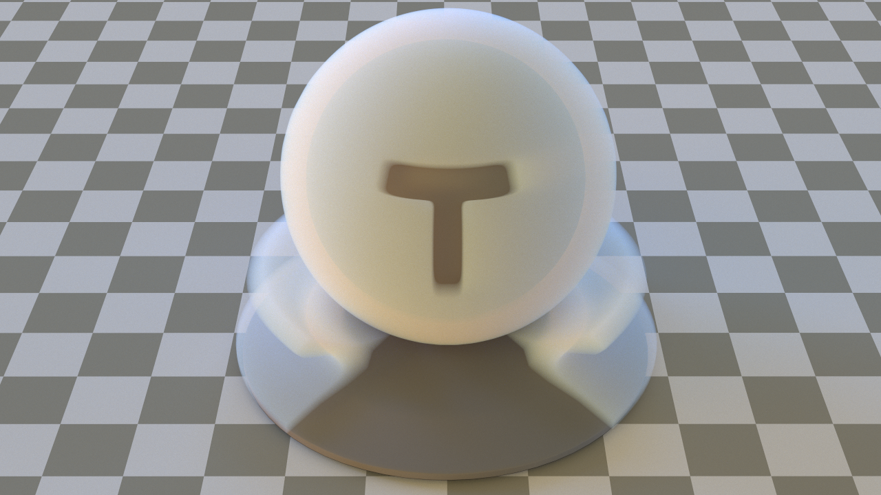
White scattering medium
Tungsten render without tonemapping

Mitsuba render
Atmospheric medium
The main purpose of the atmospheric medium is to mimic the appearance of an Earth-like atmosphere. For this purpose, it uses the Rayleigh phase function and a scattering coefficient computed using the Rayleigh scattering cross section. The real density distribution of Earth's atmosphere is approximated with an exponential distribution that reaches 1 at the surface and drops off with distance. The falloff can be further controlled to result in larger or more concentrated atmospheres.
Evaluating the transmittance of the atmospheric medium turned out to be very difficult. The integral that describes the transmittance of a ray at origin  in direction
  within the segment
  for an atmosphere centered around the origin is
 Where
Where  is the falloff scale of the atmosphere,
  is the radius of the planet and
  is the scattering coefficient at sea level.
Unfortunately, no closed-form solution exists for this integral. In "Precomputed Atmospheric Scattering", Eric Bruneton mentions an approximate fit for  , but unfortunately it is not stable for the scales that the medium is used for.
Due to the lack of closed-form solutions, I turned to numeric integration to compute the integral. Due to the rotational symmetry of the distribution, we can rewrite the above equation as
 with
with
 and
and
 The real challenge is to compute
  in a robust manner. The difficulty is that the integrand can be quite vicious - for an Earth-like atmosphere, the density drops below
  at 100km above the ground. However, if we render an image from a space-like view with the entire earth fitting into frame, the camera sits between 30'000-50'000 kilometers above ground! Due to the extremely narrow peak of the integrand, any naive raymarching or woodcock tracking based algorithm will either fail miserably or take enormous amounts of processing time to compute the result of the integral to within a reasonable error.
The graph below shows the problem: The density of the atmosphere is plotted as a function of distance along a ray. The ray is shot from a camera resting in space towards earth; it just barely grazes the earth's surface before flying off back into space. Note the extremely narrow peak of the density:
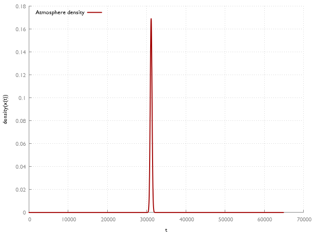
Atmosphere density along a worst-case ray
In the early steps of my implementation, this was a huge problem - the Earth's atmosphere that I wanted for my final image was nearly unrenderable due to the difficult integrand. Ultimately, I decided to go with raymarching, and it was clear that I needed some form of adaptive step size.
For the derivation of the adaptive step size, we can use the fact that the integrand consists of two monotonic parts. Using this, I devised the following constraint on the step size  at position
  along the ray
 where
where  is the integrand and
  is some user defined error threshold. In other words, for the error to stay below some bound, we wish that the function value at the next step is not "too different" from the current value, which is a reasonable constraint for a monotonic function. We can now perform a Taylor expansion of
  with respect to
  around
  and truncate it after the first term. This gives us a linear extrapolation of
  :
:
 Which we can rewrite to
 This way we can compute the adaptive step size of the ray marching algorithm using the derivative of the integrand and a user defined error threshold. Note that the derivative of the integrand is

Unfortunately, even with more sophisticated ray marching, rendering the atmospheric medium remains challenging. The strongly spectrally varying scattering coefficient combined with the exponential volume density and a high scattering albedo creates immense amounts of noise in the distance sampling step, despite MIS-ing all the color channels. I was not able to find a clever way to remedy this issue, and I had to fall back on a brute force solution: During the first interaction of a ray with the volume, one of the color channels is randomly selected and used for distance sampling. The throughput for the other color channels is set to zero. The throughput of the selected color channel has to be increased to account for the lost energy, but the technique remains unbiased. This is successful in removing most of the variance of the distance sampling step, but it comes at a cost: We are essentially multiplying the variance of all paths interacting with the volume by the number of color channels. This results in speckled noise across the color channels that is much worse than noise in the luminance.
I was not able to find a better solution to this issue, and rendering an atmospheric volume generally requires a lot more samples than a homogeneous volume of similar density. However, this finally enabled the rendering of atmospheres within a reasonable time frame! The image below shows a simple, lambertian sphere enclosed in an atmospheric medium, lit by a directional light source. Note the straight falloff in the shadow region: This is the volumetric shadow of the Earth, or, in other words, a sunset.
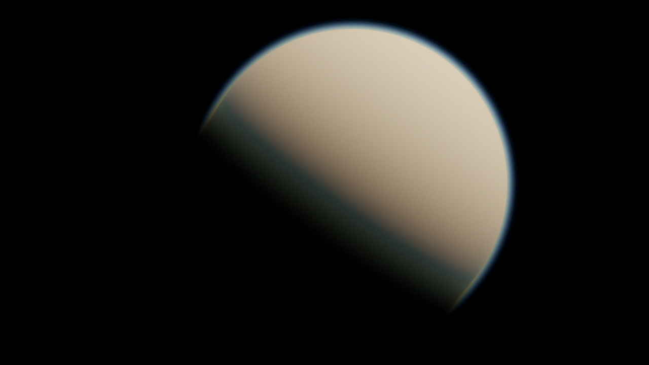
Atmosphere lit by a directional light source
Another feature I implemented for the atmospheric medium were volumetric clouds. It is clear that fully general, grid-based clouds would be very expensive, but for the special case of volumetric clouds seen from space, I implemented a simplified model instead.
Rather than requiring a voxel grid, the atmospheric medium uses a height map instead. The clouds are modeled as being contained within a thin shell bounded by two concentric spheres centered around the planet. The height map then describes the height of the clouds relative to the inner sphere. Clouds are modeled as white media with constant density. Due to the heterogeneous volume being bounded by two concentric spheres, raymarching the volume becomes fairly efficient and we can integrate clouds with the rest of the atmosphere without too much extra cost. The image below shows the same setup as before, except with an added layer of clouds:
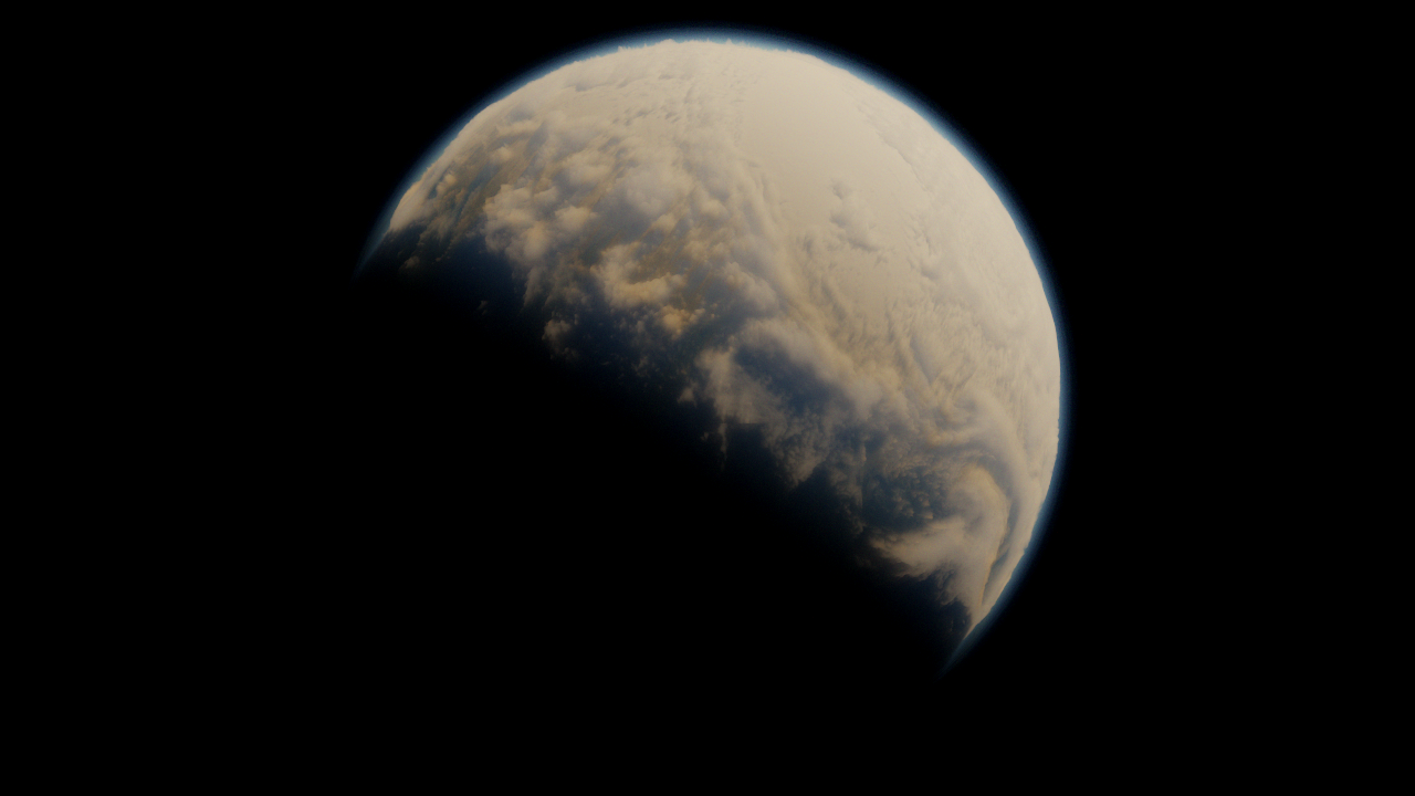
Atmosphere with volumetric clouds
Phase functions
Currently, three different phase functions are implemented. They are listed below, together with an example image:
Isotropic phase function

Bluish scattering medium with isotropic phase function

Tungsten render without tonemapping
Mitsuba render
Henyey-Greenstein phase function
Bluish scattering medium with forward scattering Henyey-Greenstein phase function (g=0.8)
Tungsten render without tonemapping
Mitsuba render
Bluish scattering medium with backward scattering Henyey-Greenstein phase function (g=-0.8)
Tungsten render without tonemapping
Mitsuba render
Rayleigh phase function
This implementation is based on the paper "Importance sampling the Rayleigh phase function" by Jeppe Frisvad. Note that this phase function is not verified with Mitsuba, since Mitsuba's implementation of the Rayleigh phase function is faulty.
Bluish scattering medium with Rayleigh phase function
Noise reduction strategies
Unfortunately, VPT tends to add significant amounts of noise under difficult lighting and high albedo, making media very expensive to use. To battle noise, I implemented various noise reduction strategies and tricks to reduce the noise footprint of media.
Direct light sampling and MIS
Direct light sampling is an immensely useful method to reduce noise under high frequency lighting. Rather than relying on phase function sampling to hit emissive surfaces, points on light sources are sampled explicitly and connected with the scattering location. Similar to surfaces, we now have two sampling strategies to sample direct lighting: Phase function sampling and light sampling. Considering only one or the other can lead to noise if either lighting or phase function is peaked. Instead, my implementation combines phase function sampling and light sampling with MIS to achieve good results.
The images below show the effect of light sampling. The first image shows a medium with high albedo at 16 spp without light sampling. The second image shows the same scene with light sampling:
Bluish scattering medium without direct light sampling

Bluish scattering medium with direct light sampling
These images show the effect of MIS for a medium with strong forward scattering (g=0.9). The first image is with light sampling only, whereas the second image shows light sampling and phase function sampling combined with MIS:
Bluish forward scattering medium without MIS
Bluish forward scattering medium with MIS
Generalized shadow rays and the forward BSDF
One important ingredient in direct light sampling is the concept of shadow rays. When we connect a point on the light source with a shading point, be it in a volume or on a surface, we have to compute whether the points are mutually visible. In a naive path tracer, the answer to this question is binary: Yes if there is no occluder, No if there is any occluder in between.
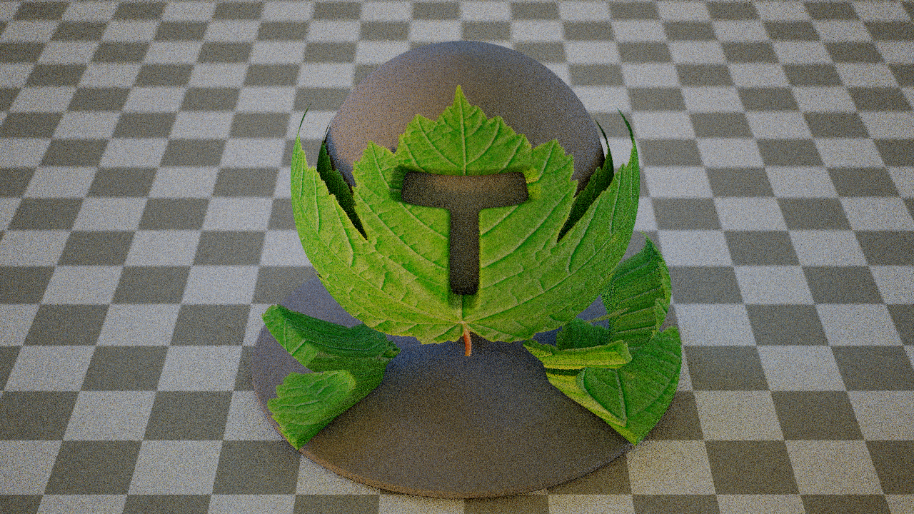
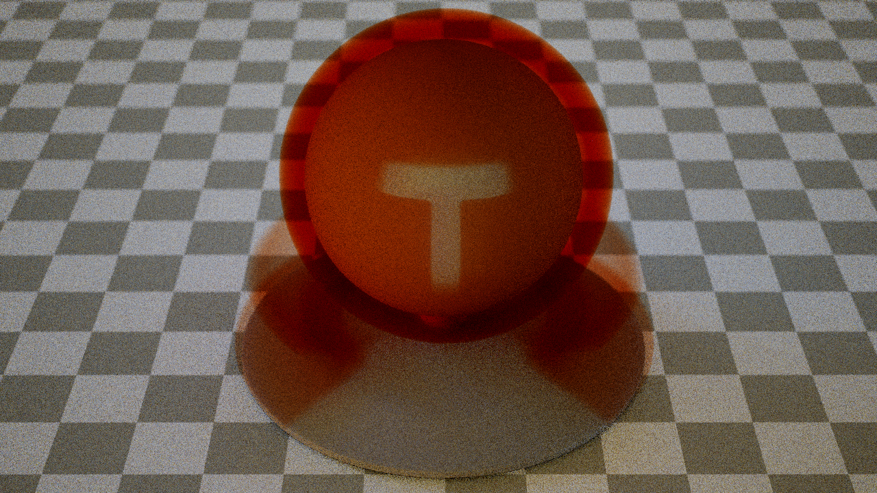
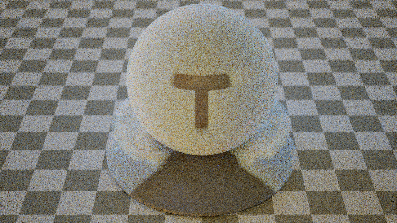
However, once we introduce transparency and volumes into the equation, a binary shadow ray may not be so ideal anymore. Here are three images of an alpha masked surface, an absorbing medium and a scattering medium with binary shadow rays:
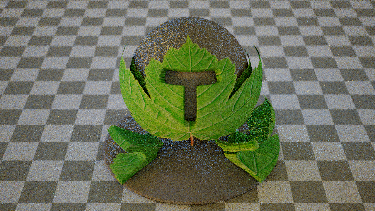
Alpha masked surface with binary shadow rays
Red absorbing medium with binary shadow rays
Bluish scattering medium with binary shadow rays
What is happening? First of all, the alpha mask does not actually remove the surface, it just makes it very transmissive - therefore, a binary shadow ray will report it as an occluder. In a similar vein, light can transmit through a medium, but the binary shadow ray will report the boundary as an occluder and thwart any attempt at light sampling in- or through the volume.
This poor shadow ray implementation can make many scenes so noisy that rendering them becomes infeasible. A simple tree with alpha masked leaves or a mildly foggy exterior can completely break the renderer. This is obviously not ideal, which is why I decided to implement generalized shadow rays; that is, shadow rays that are capable of punching through transparent surfaces and volumes and return a spectral transmission value instead of a binary result.
For media, there is some amount of cooperation required from the user, however. It is clear that not even a generalized shadow ray can sample lights through a dielectric interface - the shadow ray must be able to continue in a straight line. In general, when encountering a surface, the shadow ray cannot ignore the BSDF and simply continue in a straight line. To be able to sample lights from within a volume across the boundary surface, the surface must use the specialized Forward BSDF. When a surface is using this BSDF, the shadow ray is signaled that it can continue across the boundary. Only surfaces coated with this BSDF permit light sampling between media on either side.
Using the generalized shadow rays on the above scenes results in these images, which are much improved:
Alpha masked surface with generalized shadow rays
Red absorbing medium with generalized shadow rays
Bluish scattering medium with generalized shadow rays
The thin sheet BSDF
Sadly, if we want to be able to use light sampling in a scattering medium, we cannot use a dielectric BSDF on the boundary. This is not ideal, since many scattering media in real life are bounded by a dielectric surface. Even without participating media, many indoor scenes feature glass windows and other dielectric surfaces that contribute significantly to the light transport. Since even generalized shadow rays can't handle these BSDFs, scenes like these would suffer from considerable amounts of noise. To battle this phenomenon, I implemented a special kind of dielectric BSDF: The thin sheet BSDF.
The thin sheet BSDF models an extremely thin surface bounded by two dielectric interfaces. It is assumed that the relative index of refraction on both interfaces is the same. Since the surface is very thin, we can also make the approximation that all light exits at the same location as it entered. With this setup, we can analytically compute the amount of light that is reflected and transmitted through the surface via all possible scattering events through a geometric series.
We can implement the thin sheet model as a simple BSDF with both a specular reflection and a specular transmission component. However, we can do much better: Since the transmitted direction is the same as the incident direction, we can also implement the thin sheet BSDF as a mirror BSDF with an angle dependent transparency value. The difference is subtle, but since the latter implementation uses transparency instead of specular transmission, it actually allows for generalized shadow rays to punch through thin sheet surfaces!
This means that we can actually render indoor scenes with lots of glass windows and scattering media with a thin dielectric interface without paying the cost of excessive noise. The thin sheet approximation only roughly mimics a true dielectric interface, but it is much better than not having an interface at all. In most practical situations, the unsuspecting audience might not even notice that an interface is not truly dielectric.
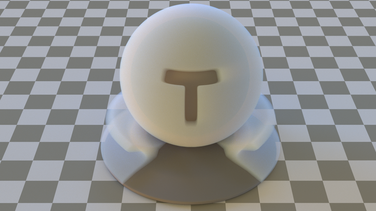
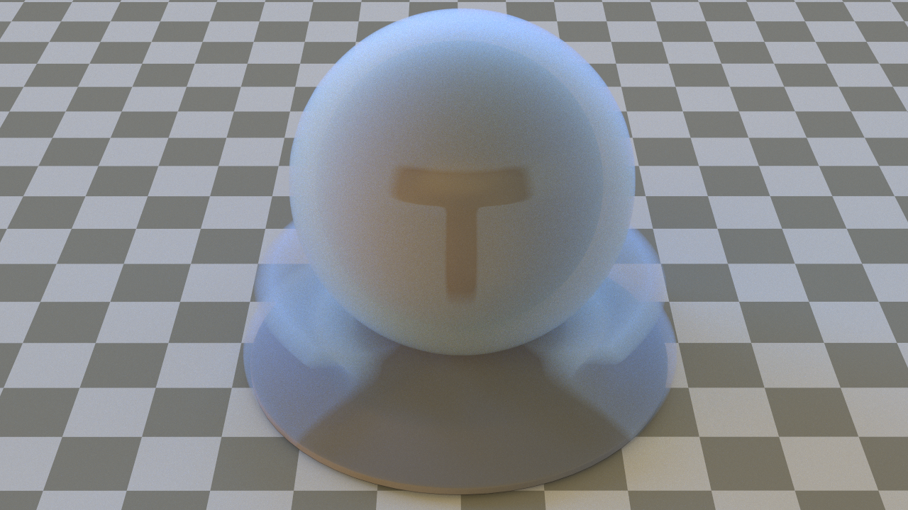
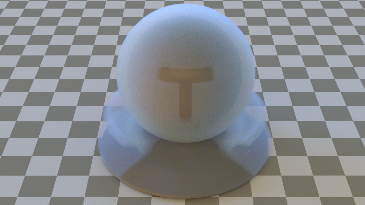
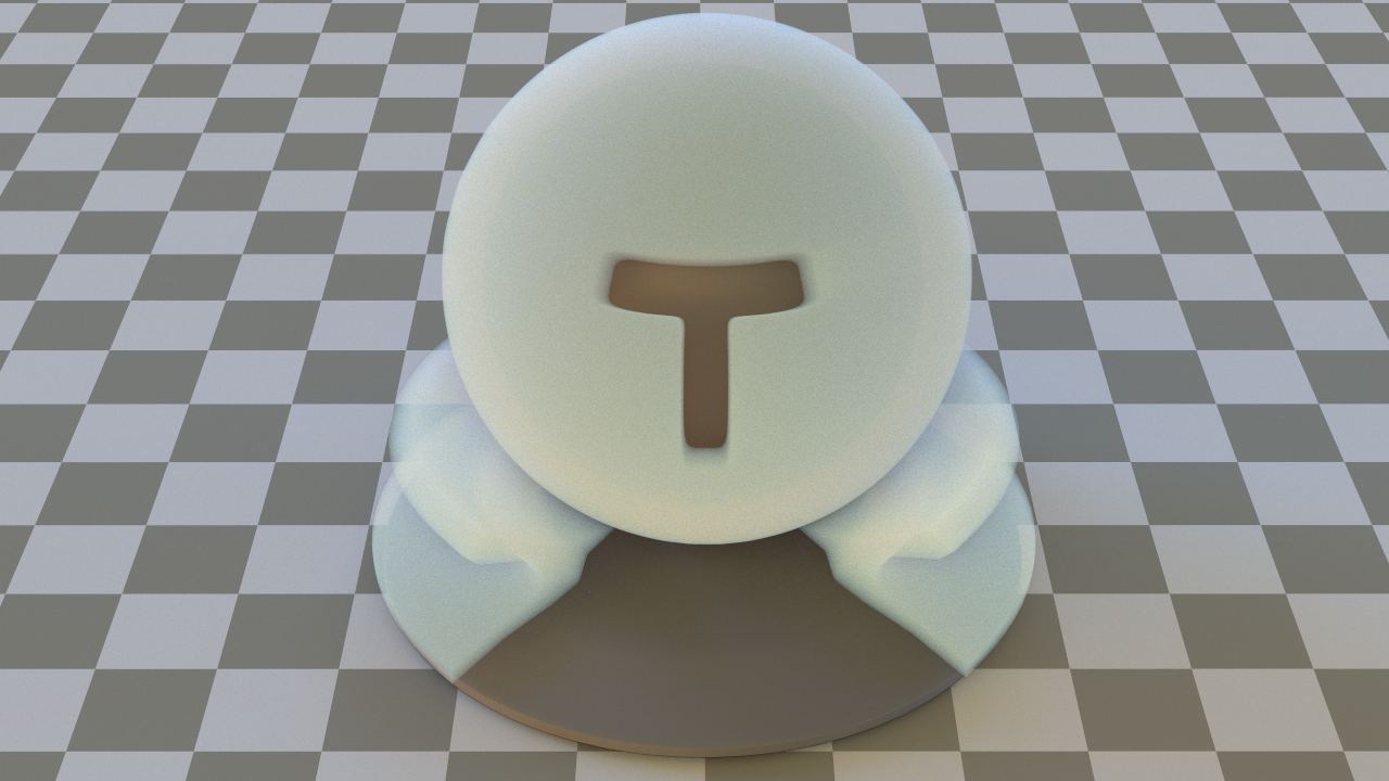
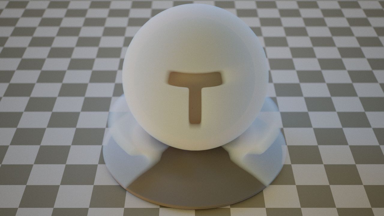
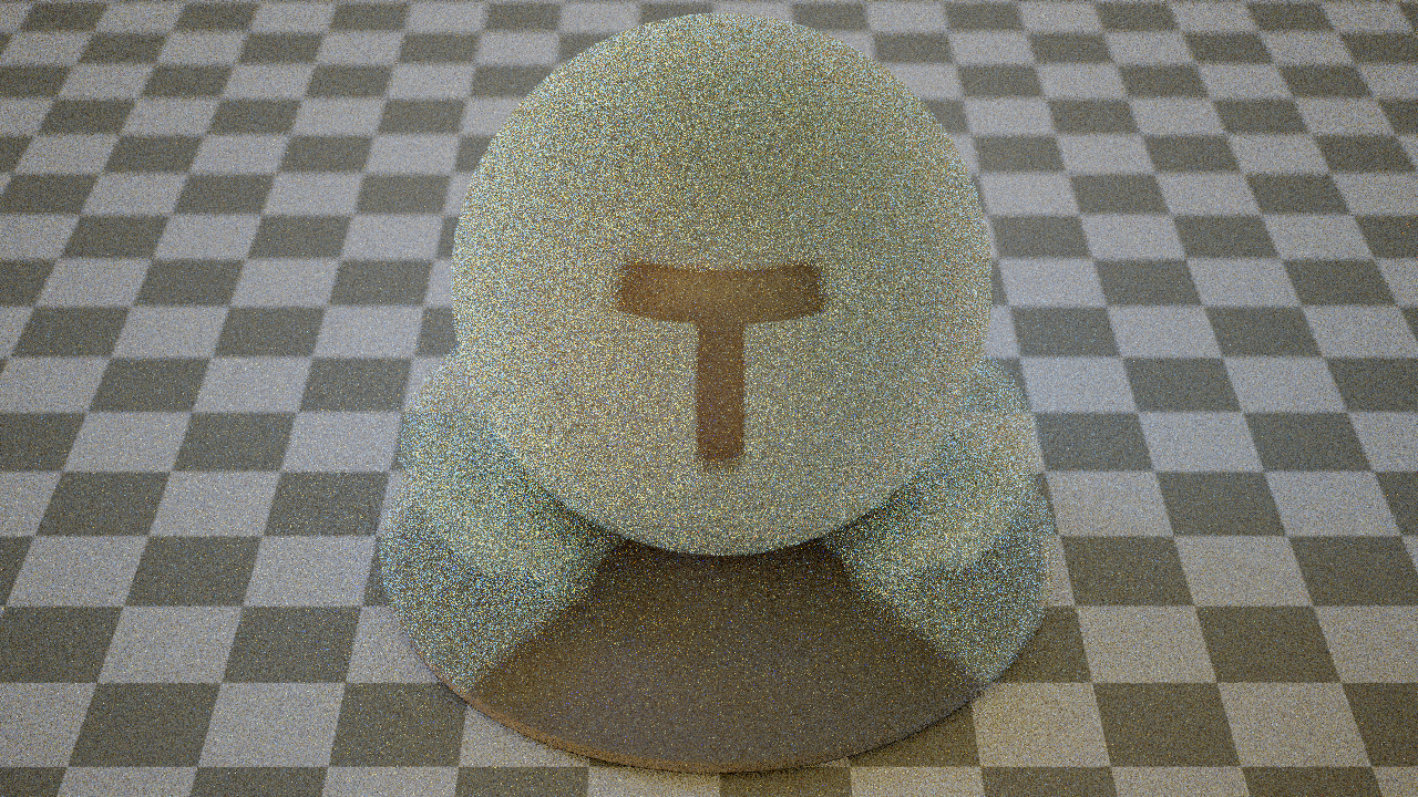
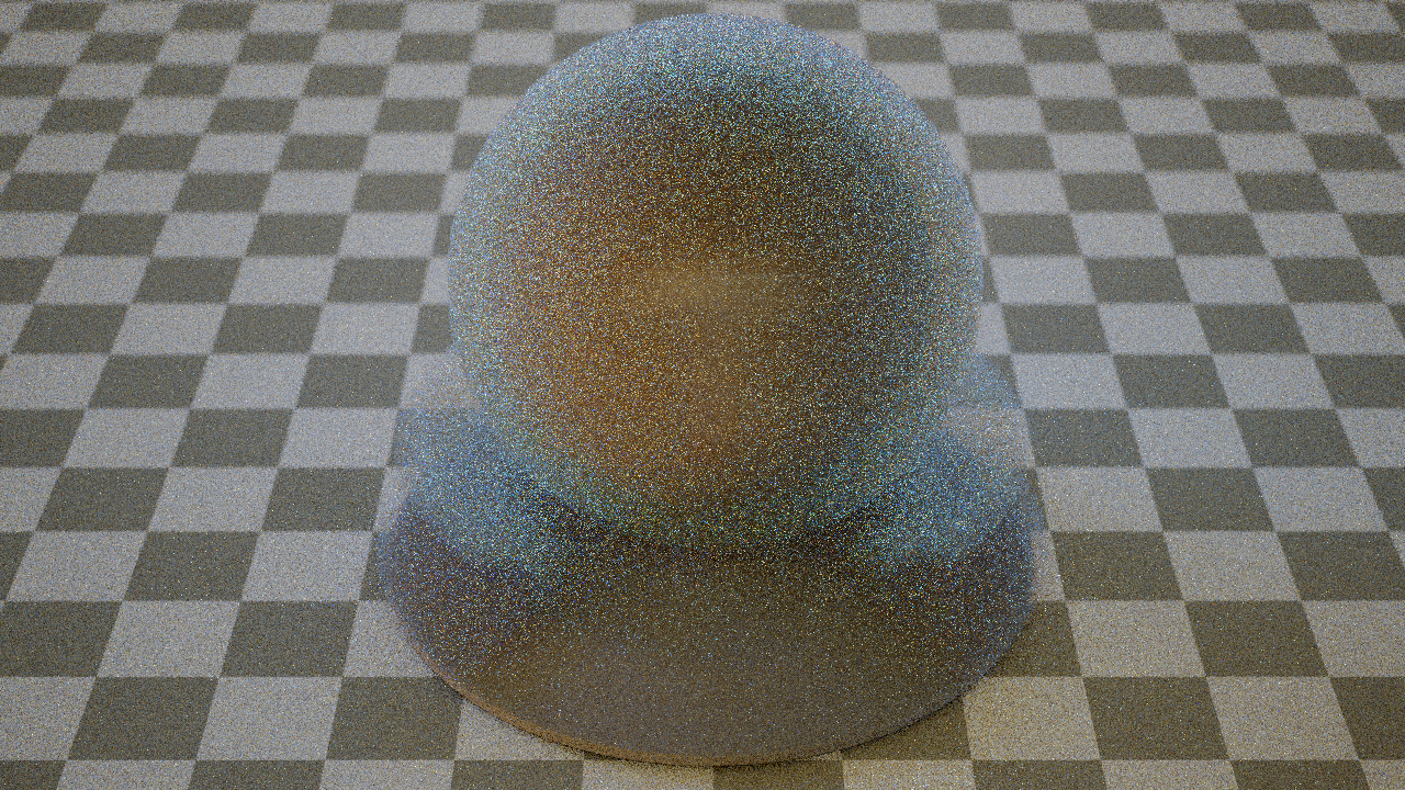
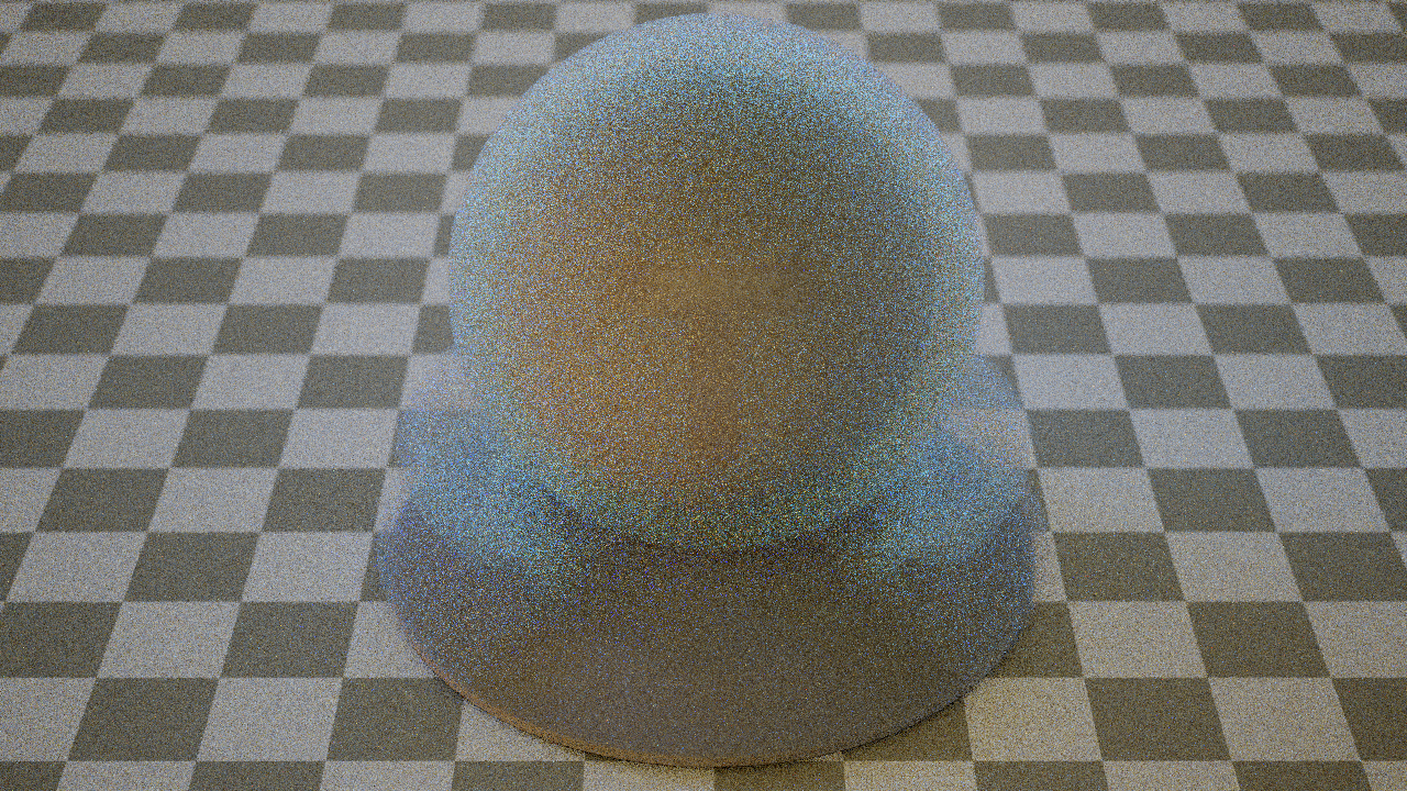
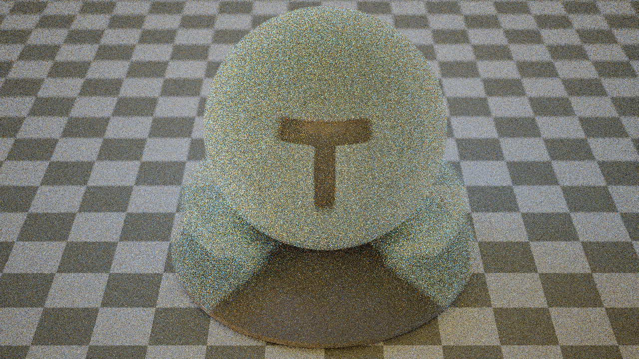
Below are four renders of a thin sheet BSDF: The first two show an object with a thin glass shell, the second two a thin glass shell filled with a scattering medium. In both scenes, one image shows the naive thin sheet BSDF and one image shows the improved implementation using the transparency trick. All scenes rendered at 64 spp. Note the difference in noise:

Naive thin sheet BSDF
Shadow ray friendly thin sheet BSDF
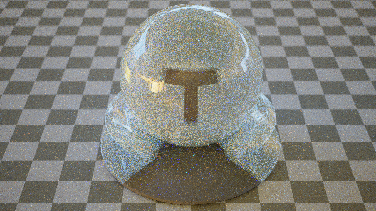
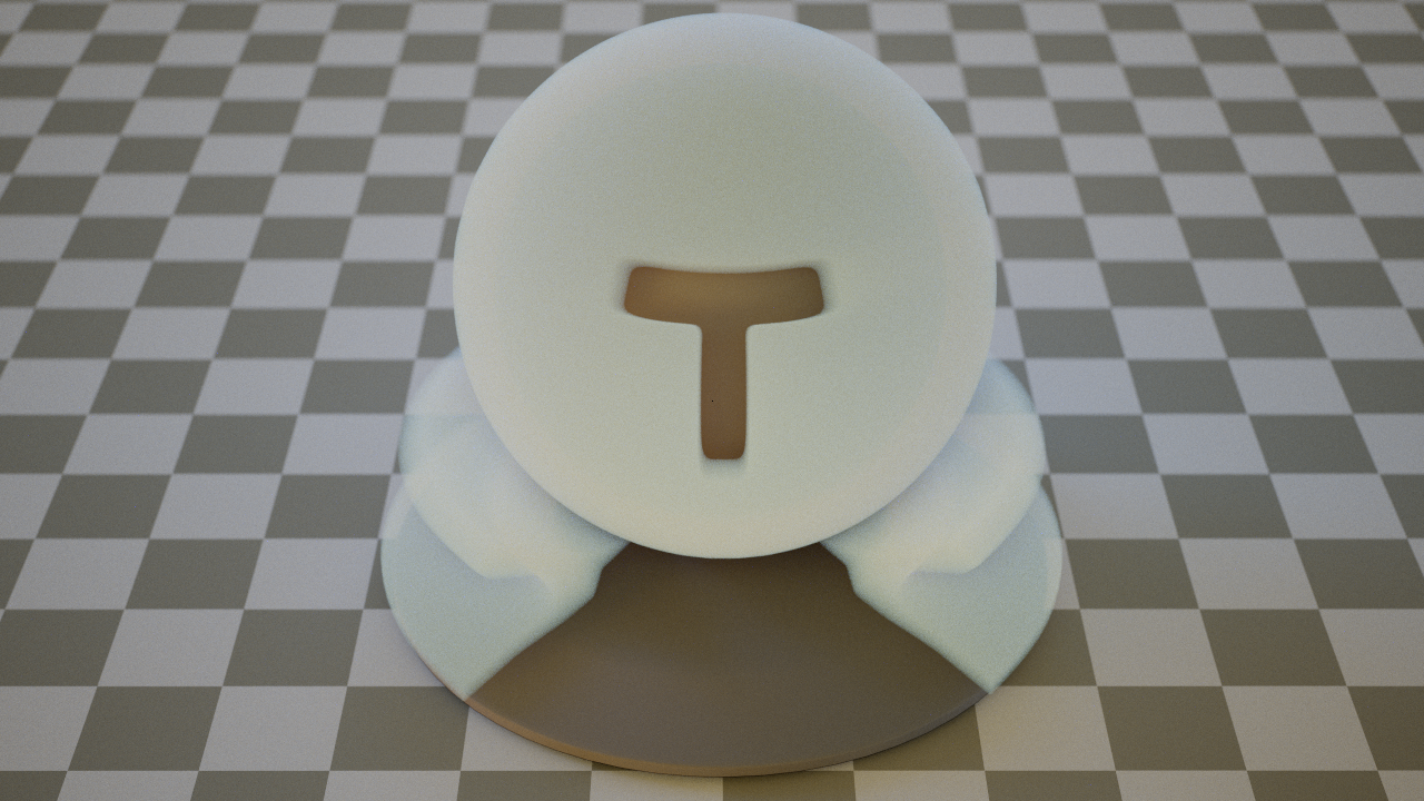
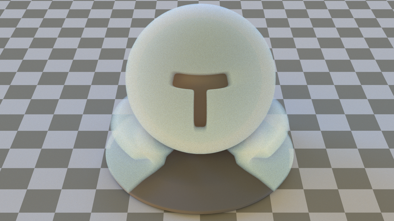
Bluish scattering volume encased by a naive thin sheet BSDF
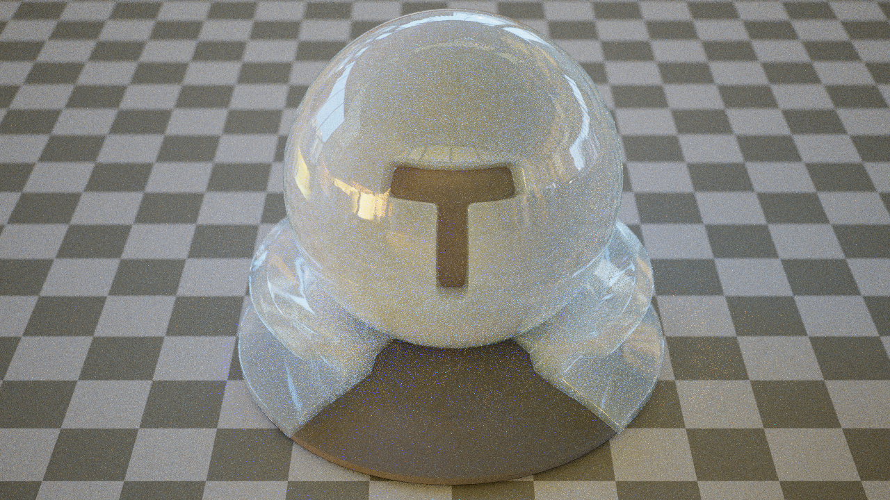
Bluish scattering volume encased by a shadow ray friendly thin sheet BSDF
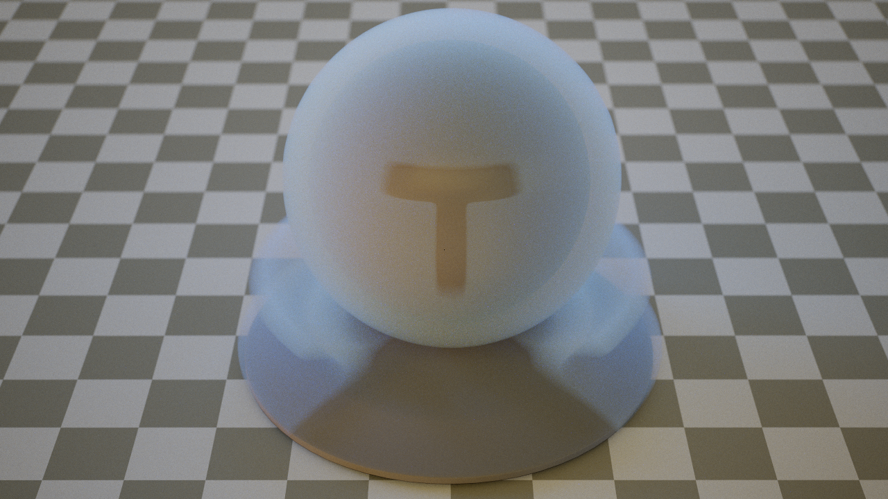
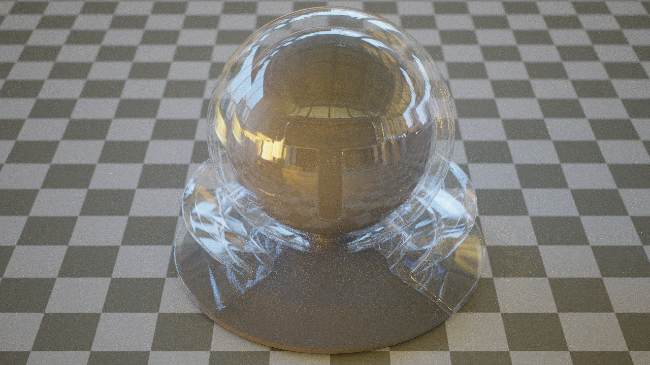
And finally, here's a converged image of a thin sheet BSDF with high index of refraction at 2048spp:
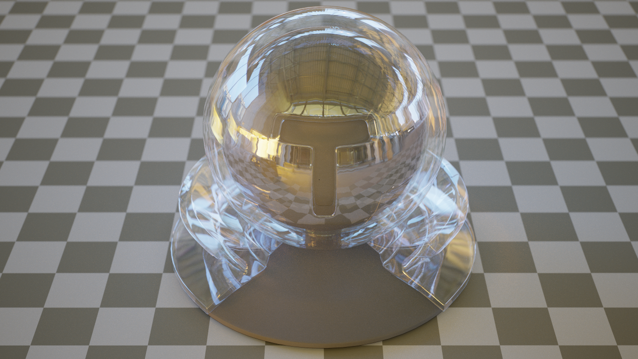
Converged thin sheet BSDF